
4.6 Level Crossing and Balance Equations
Consider a sample path of \(\{\L(t) : t\geq 0\}\) of a queueing or inventory system in which jobs arrive and depart one by one. We say that the sample path up-crosses level \(n\) at time \(t\) when the number of jobs in the system changes from \(n\) to \(n+1\) due to an arrival, that is, when \(L(t-)=n\) and \(L(t)=n+1\). The sample path down-crosses level \(n\) at time \(t\) when, due to a departure, \(L(t-)=n+1\) and \(L(t)=n\). Clearly, the number of up-crossings and down-crossings cannot differ by more than 1 at any time, because a down-crossing of level \(n\) can only occur after an up-crossing (or the other way around). This simple idea is a key tool in the analysis of stationary stochastic systems.
Similar to the definitions for \(A(n,t)\) and \(\lambda(n)\), let1 Note that we write \(L(D_{k})\) and not \(L(D_{k}-)\): to leave \(n\) jobs behind, the system must contain \(n+1\) jobs just prior to the departure.
\begin{align*} D(n,t) &:= \sum_{k=1}^{D(t)} \1{\L(D_k) = n}, & \mu(n+1) := \lim_{t\to\infty} \frac{D(n,t)}{Y(n+1,t)}, \tag{4.6.1} \end{align*}denote the number of departures up to time \(t\) that leave \(n\) jobs behind, and the departure rate from state \(n+1\).
When jobs arrive and depart as single units and the limits Eq. (4.5.1) and Eq. (4.6.1) hold,
\begin{equation*} \lambda(n) p(n) = \mu(n+1)p(n+1). \tag{4.6.2} \end{equation*}
Proof
Since jobs arrive one by one, \(|L(t) - L(t-)| \leq 1\) for all \(t\geq 0\). This implies that
\begin{equation*} |A(n,t) - D(n,t)| \leq 1, \tag{4.6.3} \end{equation*}hence,
\begin{equation*} \lim_{t\to\infty} \frac{A(n,t)}t = \lim_{t\to\infty} \frac{D(n,t)}t. \tag{4.6.4} \end{equation*}The claim follows by noting that
\begin{align*} \lim_{t\to\infty} \frac{A(n,t)}t &= \lim_{t\to\infty} \frac{A(n,t)}{Y(n,t)}\frac{Y(n,t)}t = \lambda(n) p(n),\\ \lim_{t\to\infty} \frac{D(n,t)}t &= \lim_{t\to\infty} \frac{D(n,t)}{Y(n+1,t)}\frac{Y(n+1,t)}t = \mu(n+1) p(n+1). \end{align*}Suppose we can specify2 In Section 5.1 and onward we will model many queueing situations by making suitable choices for \(\lambda(n)\) and \(\mu(n)\). the arrival and service rates \(\lambda(n)\) and \(\mu(n)\), then we can easily compute the long-run fraction of time \(p(n)\) that the system contains \(n\) jobs. To see this, rewrite Eq. (4.6.2) as
\begin{equation*} p(n+1) = \frac{\lambda(n)}{\mu(n+1)}p(n). \tag{4.6.5} \end{equation*}A simple recursion yields:
\begin{equation*} p(n+1) = \frac{\lambda(n)\lambda(n-1)\cdots \lambda(0)}{\mu(n+1)\mu(n)\cdots \mu(1)}p(0). \end{equation*}Since \(p(n)\), \(n\geq 0\), represent probabilities,
\begin{equation*} 1 = \sum_{n=0}^\infty p(n)= p(0)\left(1+\sum_{n=0}^\infty \frac{\lambda(n)\lambda(n-1)\cdots\lambda(0)}{\mu(n+1)\mu(n)\cdots \mu(1)}\right). \end{equation*}Thus, we can normalize \(p(n)\) by setting
\begin{equation*} p(0)^{-1} = 1+\sum_{n=0}^\infty \frac{\lambda(n)\lambda(n-1)\cdots\lambda(0)}{\mu(n+1)\mu(n)\cdots \mu(1)} \tag{4.6.6} \end{equation*}Finally, once we have \(p(n)\), it is easy to compute the time-average number of jobs in the system and the long-run fraction of time it contains at least \(n\) jobs:
\begin{align*} \E\L &= \sum_{n=0}^\infty n p(n), & \P{\L \geq n} &= \sum_{i=n}^\infty p(i). \end{align*}With the definitions of \(A(n,t)\) and \(D(n,t)\), we establish a relation between \(\pi(n)\) and \(\delta(n)\), i.e., statistics as obtained by arrivals and departures. Define, analogous to \(\pi(n)\),
\begin{equation*} \delta(n) := \lim_{t\to\infty} \frac{D(n,t)}{D(t)} \end{equation*}as the long-run fraction of jobs that leave \(n\) jobs behind. From Eq. (4.6.4) and using that \(A(n,t) \approx D(n,t)\),
\begin{equation*} \frac{A(t)}t \frac{A(n,t)}{A(t)} = \frac{A(n,t)}t \approx \frac{D(n,t)}t = \frac{D(t)}t \frac{D(n,t)}{D(t)}. \end{equation*}Taking limits at the left and right, and using Eq. (4.1.1), we obtain for the \(G/G/c\) queue3 Because customers arrive and leave as single units in a (rate-stable) \(G/G/c\) queue.
\begin{equation*} \lambda \pi(n) = \delta \delta(n). \tag{4.6.7} \end{equation*}Hence,
\begin{equation*} \lambda = \delta \iff \pi(n) = \delta(n). \tag{4.6.8} \end{equation*}When jobs can be blocked, we must distinguish between jobs that arrive and those that actually enter.4 Blocked jobs do not enter, hence do not produce up-crossings. To handle this, define
\begin{align*} A^{+}(n,t) &:= \sum_{k=1}^{A(t)} \1{L(A_k-) = n}\1{\L(A_k) \geq n+1}, & \lambda^{+}(n) &:= \lim_{t\to\infty} \frac{A^{+}(n,t)}{Y(n,t)}, \tag{4.6.9} \end{align*}i.e., \(A^{+}(n,t)\) counts arrivals that up-cross level \(n\), and \(\lambda^{+}(n)\) corresponds to the rate at which jobs enter when the system contains \(n\) jobs.5 \(\lambda(n) > \lambda^{+}(n)\) when a fraction of jobs is blocked, otherwise \(\lambda(n) = \lambda^{+}(n)\). We should replace \(\lambda(n)\) by \(\lambda^{+}(n)\) at all other relevant places, for instance, Eq. (4.6.2) becomes
\begin{equation*} \lambda^{+}(n) p(n) = \mu(n+1) p(n+1). \tag{4.6.10} \end{equation*}It is important to realize that level-crossing arguments in the simple form as presented above cannot always be applied, since it is not always possible to split the state space into two disjoint subsets by `drawing a line' between two states. For a more general approach, we focus on a single state and count how often this state is entered and left.

Specifically, define \(I(n,t) = A(n-1,t) + D(n,t)\) as the number of times the queueing process enters state \(n\) either by an arrival from state \(n-1\) or a departure leaving \(n\) jobs behind. Similarly, \(O(n,t) = A(n,t) + D(n-1,t)\) counts how often state \(n\) is left either by an arrival (to state \(n+1\)) or a departure (to state \(n-1\)). Just like Eq. (4.6.3), it is evident that \(|I(n,t)-O(n,t)|\leq 1\), and this implies6 Ex 4.6.10.
\begin{equation*} \lambda(n-1)p(n-1)+\mu(n+1)p(n+1) = (\lambda(n)+\mu(n))p(n). \tag{4.6.11} \end{equation*}These equations hold for any \(n\geq 1\) and are known as the balance equations. These equations are useful for analyzing queueing networks.
Level-crossing arguments can also be applied to continuous systems. For instance, we can find a closed-form expression for the waiting time of the \(M/G/1\) queue. However, this is a bit more complicated as the argument hinges on an integral equation. If you do not like developing mathematical skills, you may skip this derivation.
Suppose that the waiting time \(W\) of the \(M/G/1\) queue has a density \(f\), that is, the cdf \(F(x) = \P{W\leq x}\) has a derivative \(f(x)\) for all \(x>0\).7 A formal proof would first establish that \(f\) exists. , 8 At \(x=0\), \(F\) is only differentiable from the right because \(\P{W=0}>0\), while \(\P{W\leq x} = 0\) for \(x<0\). Consider some level \(x>0\). By PASTA, the rate of arriving jobs that see a waiting time \(y \in [0, x)\) is equal to \(\lambda f(y)\).9 Observe that we use the splitting property of Poisson processes. To up-cross level \(x\) from state \(y< x\), the service time must be at least \(x-y\), the probability of which is \(G(x-y) = \P{S>x-y}\). Adding up the rates for all possible waiting times below \(x\) gives that \(\lambda\int_0^x f(y) G(x-y)\d y\) is the up-crossing rate of level \(x\). The down-crossing rate equals \(f(x)\) because the server drains work at unit rate, so level \(x\) is crossed downward whenever the workload is at \(x\). Equating these rates gives the integral equation \(\lambda \int_0^{x} f(y) G(x-y)\d y = f(x)\). For \(x=0\), we need to consider the atom \(\P{W=0}\). In that case, \(\lambda \P{W=0} = f(0+)\). We can combine these observations into the following level-crossing equation:
\begin{equation*} \lambda\int_0^x G(x-y) \d F(y) = f(x). \tag{4.6.12} \end{equation*}Using this integral equation
\begin{align*} \E W &= \int_0^{\infty} x f(x) \d x = \lambda \int_0^{\infty} x \int_0^{x} G(x-y) \d F(y) \d x \\ &= \lambda \int_0^{\infty} \int_0^{\infty} x \1{y \leq x} G(x-y) \d x \d F(y) \\ &= \lambda \int_0^{\infty} \int_0^{\infty} (u+y) G(u) \d u \d F(y) \\ &\stackrel 1 = \lambda \int_0^{\infty} (\E{S^2}/2 + y \E S) \d F(y) \\ &\stackrel 2= \lambda \E{S^2}/2 + \lambda \E S \E \W. \end{align*}Step 1 follows from substituting \(u=x-y\), and 2 from the fact that \(\E \W = \int_{0}^{\infty} y \d F (y)\). Bringing the term \(\lambda \E S \E \W = \rho \E \W\) to the left, and dividing by \(1-\rho\) gives
\begin{align*} \E \W &= \lambda \frac{\E{S^2}}{2(1-\rho)}. \end{align*}As a last point of interest, let us derive the density of the waiting time for the \(M/M/1\) queue. As in this case \(S\sim \Exp{\mu}\), \(f\) must satisfy
\begin{align*} f(x) = \lambda \int_0^x e^{-(x-y)\mu} \,\d F(y) = \lambda \int_0^x e^{-(x-y)\mu} f(y) \d y + \lambda e^{-x \mu} F(0). \end{align*}Multiplying both sides by \(e^{\mu x}\) and defining \(g(x) = e^{\mu x} f(x)\), this can be rewritten to \(g(x) = \lambda \int_0^x g(y) \d y + \lambda F(0)\). Differentiating the LHS and RHS with respect to \(x\) gives the differential equation \(g'(x) = \lambda g(x)\). Hence, \(g(x) = A e^{\lambda x}\), and therefore, \(f(x) = A e^{-(\mu-\lambda)x}\). At \(x=0\), \(f(0) = \lambda \P{W=0} = \lambda p(0)\). Since \(p(0)=1-\rho\), it follows that
\begin{equation*} f(x) = \lambda(1-\rho) e^{- \mu(1-\rho)x}, \quad x > 0. \tag{4.6.13} \end{equation*}Another way to obtain this result is to condition on the number \(\L\) of jobs found upon arrival, and then using that the total service of these \(\L\) customers has a gamma density:10 If \(L(t) = k > 0\), the new arrival finds one job at the server and \(k-1\) in queue. Each of these jobs in the system has to be served before it is the turn of the new job.
\begin{align*} f(x) &= \sum_{k=1}^\infty \P{W = x | \L = k}\P{\L = k } \\ &= \sum_{k=1}^\infty \P{S_1 + S_2 + \cdots + S_k = x}\P{\L = k } = (1-\rho) \sum_{k=1}^\infty \rho^k \mu \frac{(\mu x)^{k-1}}{(k-1)!}e^{-\mu x}\\ &= (1-\rho) \lambda e^{-\mu x}\sum_{k=0}^\infty \rho^{k} \frac{(\mu x)^{k}}{k!} = (1-\rho) \lambda e^{-\mu (1-\rho)x}. \end{align*}In a large hotel, taxis arrive at a rate of \(\lambda = 15\) per hour and riders' parties arrive at a rate of \(\mu=12\) per hour. Whenever taxis are waiting, riders are served immediately upon arrival. Whenever riders are waiting, taxis are loaded immediately upon arrival. A maximum of three taxis can wait at a time (other cabs must go elsewhere). Let \(p(i,j)\) be the steady-state probability that there are \(i\) parties of riders and \(j\) taxis waiting at the hotel. Claim: the transitions are modeled by the graph below.

Solution
Solution, for real
True.
Claim: To obtain balance equations, we do not count the number of up- and down-crossings of a level. Instead, we count how often a box around a state, such as state \(2\) in the figure below, is crossed from inside and outside.
Solution
Solution, for real
True.
Consider the \(M^2/M^2/1/3\) queue. The graph below shows all relevant transitions.

Solution
Solution, for real
False. The figure sketches the \(M/M^2/1/3\) queue.
For the \(G/G/1\), the difference between the number of `out-transitions' and the number of `in-transitions' is at most 1 for all \(t\). As a consequence,
\begin{align*} \text{transitions out } &\approx \text{transitions in } \iff \\ A(n,t) + D(n-1,t) &\approx A(n-1,t) + D(n,t) \iff \\ \frac{A(n,t) + D(n-1,t)}t &\approx \frac{A(n-1,t) + D(n, t)}t \iff \\ \frac{A(n,t)}t + \frac{D(n-1,t)}t &\approx \frac{A(n-1,t)}t + \frac{D(n,t)}t. \end{align*}Thus, under proper technical assumptions (which you can assume to be satisfied) this becomes for \(t\to\infty\),
\begin{equation*} (\lambda(n) +\mu(n))p(n) = \lambda(n-1)p(n-1) + \mu(n+1)p(n+1). \end{equation*}We claim that if we specialize this result for the \(M/D/1\) queue we get \(\lambda(n) = \lambda\) and \(\mu(n) = \mu\), hence using PASTA,
\begin{equation*} (\lambda +\mu)\pi(n) = \lambda\pi(n-1) + \mu\pi(n+1). \end{equation*}Solution
Solution, for real
False. Since service times are constant in the \(M/D/1\) queue and thus not memoryless, \(\mu \neq \mu(n+1)\) for the \(M/D/1\) queue.
Claim: The level-crossing equation \(\lambda(n)p(n) = \mu(n+1)p(n+1)\) holds for any queueing system in which jobs arrive and depart one at a time.
Solution
Solution, for real
True. When jobs arrive and depart as single units, the number of up-crossings and down-crossings of any level \(n\) can differ by at most one, leading to this equation in the long run.
Consider the following (silly) queueing process. At times \(0, 2,4, \ldots\) customers arrive, each customer requires \(1\) unit of service, and there is one server.
- Find an expression for \(A(n,t)\), when \(L(0)=0\).
- Show that \(\pi(0)=1\) and \(\pi(n)=0\), for \(n>0\).
- Check that \(\lambda \pi(n) = \lambda(n) p(n)\).
- Find an expression for \(Y(n,t)\).
- Compute \(p(n)\) and \(\lambda(n)\).
- Compute \(D(n,t)\) and \(\mu(n+1)\) for \(n\geq 0\).
- Compute \(\lambda(n) p(n)\) for \(n\geq 0\), and check \(\lambda(n) p(n) = \mu(n+1) p(n+1)\).
Solution
Solution, for real
- \(A_{k} = 2(k-1)\), \(k=1, 2, \ldots\), as jobs arrive at \(t=0, 2, 4, \ldots\) Thus, \(A(t) = 1 + \lfloor t/2 \rfloor\) for \(t \geq 0\).
(BTW, \(A(t)/t \to 1/2\) as \(t\to \infty\).) We also know that \(L(s)=1\) if \(s\in [2k, 2k+1)\) and \(L(s)=0\) for \(s\in[2k-1, 2k)\) for \(k=0, 1, 2, \ldots\). Thus, \(L(A_k-) = L(2k-)=0\). Therefore, \(A(0,t) = A(t)\) for \(t \geq 0\), and \(A(n,t)=0\) for \(n\geq 1\).
- All arrivals see an empty system. Hence, \(A(0,t)/A(t) \approx (t/2)/(t/2) = 1\), and \(A(n,t)=0\) for \(n>0\). Thus, \(\pi(0) = \lim_{t\to\infty} A(0,t)/A(t) = 1\) and \(\pi(n)=0\) for \(n>0\). Recall from the other exercises that \(p(0)=1/2\). Hence, statistics as obtained via time-averages are not necessarily the same as statistics obtained at arrival moments (or any other point process).
- \(\lambda = \lim_{t\to\infty} A(t)/t = 1/2\). \(\lambda(0)=1\), \(p(0)=1/2\), and \(\pi(0)=1\). Hence,
For \(n>0\), the argument is straightforward: everything is 0.
Observe that the system never contains more than 1 job. Hence, \(Y(n,t)=0\) for all \(n\geq 2\). Then we see that \(Y(1,t) = \int_0^t \1{\L(s) = 1}\d s\). Now observe that for our queueing system \(L(s)=1\) for \(s\in[0,1)\), \(L(s)=0\) for \(s\in[1,2)\), \(L(s)=1\) for \(s\in[2,3)\), and so on. Thus, when \(t<1\), \(Y(1,t)=\int_0^t \1{\L(s)=1} \d s = \int_0^t 1\d s = t\). When \(t\in[1,2)\),
\begin{equation*} L(t)=0 \implies \1{\L(t)=0} \implies Y(1,t) \text{ does not change}. \end{equation*}
Continuing to \([2,3)\) and so on gives
\begin{equation*} Y(1,t) = \begin{cases} t & t\in[0,1), \\ 1 & t\in[1,2), \\ 1+(t-2) & t\in[2,3), \\ 2+(t-4) & t\in[4,5), \end{cases} \end{equation*}and so on. With this, we see that the general formula must be
\begin{equation*} Y(1, t) = \begin{cases} \lfloor t/2\rfloor + t-\lfloor t \rfloor, &\text{if } \lfloor t \rfloor \text{ is even}, \\ 1+ \lfloor t/2\rfloor, &\text{if } \lfloor t \rfloor \text{ is odd}. \end{cases} \end{equation*}Since \(Y(n,t)=0\) for all \(n\geq 2\), \(L(s) = 1\) or \(L(s)=0\) for all \(s\), therefore,
\begin{equation*} Y(0,t) = t-Y(1,t). \end{equation*}- \begin{align*} \lambda(0) &\approx \frac{A(0,t)}{Y(0,t)} \approx \frac{t/2}{t/2} = 1, \\ \lambda(1) &\approx \frac{A(1,t)}{Y(1,t)} \approx \frac{0}{t/2} = 0, \\ p(0) &\approx \frac{Y(0,t)}{t} \approx \frac{t/2}{t} = \frac 1 2, \\ p(1) &\approx \frac{Y(1,t)}{t} \approx \frac{t/2}{t} = \frac 1 2. \end{align*}
For the rest \(\lambda(n) = 0\), and \(p(n)=0\), for \(n\geq 2\).
- \(D(0,t) = \sum_{k=1}^\infty\1{D_k\leq t, L(D_k)=0}\).
From the graph of \(\{\L(s)\}\) we see that all jobs leave an empty system behind. Thus, \(D(0,t) \approx t/2\), and \(D(n,t)=0\) for \(n\geq 1\). With this, \(D(0,t)/Y(1,t) \sim (t/2)/(t/2) = 1\), and so,
\begin{equation*} \mu(1) = \lim_{t\to\infty} \frac{D(0,t)}{Y(1, t)} = 1, \end{equation*}and \(\mu(n) = 0\) for \(n\geq2\).
- \(\lambda(0)p(0)=1\cdot 1/2 = 1/2\), \(\lambda(n)p(n)= 0\) for \(n>1\), as \(\lambda(n)=0\) for \(n>0\).
Next, \(\mu(1)=1\), hence \(\mu(1) p(1) = 1\cdot 1/2 = 1/2\). Moreover, \(\mu(n)=0\) for \(n\geq 2\). Clearly, for all \(n\) we have \(\lambda(n)p(n)= \mu(n+1)p(n+1)\).
Derive \(\E\L = \sum_{n=0}^\infty n p(n)\) from Eq. (4.2.3).
Solution
Solution, for real
Noting that \(L(s) = \sum_{n=0}^\infty n\, \1{\L(s) = n}\), we see that
\begin{equation*} \frac 1 t \int_0^t L(s) \d s = \frac 1 t \int_0^t \left(\sum_{n=0}^{\infty} n\, \1{\L(s) = n}\right) \d s = \sum_{n=0}^{\infty} \frac n t \int_0^t \1{\L(s) = n} \d s = \sum_{n=0}^{\infty} n \frac{Y(n,t)}{t} \end{equation*}Taking the limit \(t\to\infty\) and applying Eq. (4.5.1) (and reversing the limit and the summation, which we assume is okay here) we obtain that \(\E \L = \sum_{n} n p(n)\).
Show for the \(M/G/1\) that with probability \(\rho\) a job leaves behind a busy server.
Hint
Apply PASTA and Eq. (4.6.8).
Solution
Solution, for real
Use the references of the hint to see that \(\rho = \sum_{i=1}^\infty p(i) = \sum_{i=1}^\infty \pi(i) = \sum_{i=1}^\infty \delta(i)\).
Consider a single server that serves one queue and serves only in batches of 2 jobs at a time (so never 1 job or more than 2 jobs). At most 3 jobs fit in the system. Single jobs arrive as a Poisson process with \(\lambda\). Due to blocking, we set \(\lambda(n) = \lambda\) for \(n<3\) and \(\lambda(n)=0\) for \(n\geq 3\). The batch service times are exponentially distributed with mean \(1/\mu\), so that by the memoryless property, \(\mu(n) = \mu\).
Make a graph of the state-space and show, with arrows, the transitions that can occur and use level-crossing arguments to express the steady-state probabilities \(p(n), n=0,\ldots, 3\) in terms of \(\lambda\) and \(\mu\).
Solution
Solution, for real
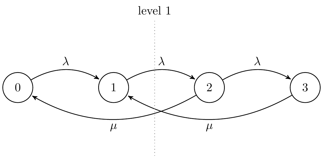
With level-crossing:
\begin{align*} \lambda p(0) &= \mu p(2), \quad\text{the level between 0 and 1,}\\ \lambda p(1) &= \mu p(2) +\mu p(3), \quad\text{see level 1,}\\ \lambda p(2) &= \mu p(3), \quad\text{the level between 2 and 3.}\\ \end{align*}Solving this in terms of \(p(0)\) gives \(p(2) = \rho p(0)\), \(p(3) = \rho p(2) = \rho^2p(0)\), and
\begin{equation*} \lambda p(1) = \mu(p(2) + p(3)) = \mu (\rho + \rho^2) p(0) = (\lambda + \lambda^2/\mu) p(0), \end{equation*}hence \(p(1) = p(0)(\mu + \lambda)/\mu\). For the final answer, use the normalization constraint \(p(0) + p(1) + p(2) + p(3)= 1\). (As this is simple, we skip it.)
Note that the figure tells what type of transitions (that is, jumps from one state to another) are allowed, and the rate (that is, the inverse of the expected time of the exponential time the system remains in a state). It does not imply that, once a state is entered, the state will be left immediately.
Show Eq. (4.6.11) from \(|I(n,t)-O(n,t)|\leq 1\).
Solution
Solution, for real
and
\begin{equation*} \lim_{t\to\infty} \frac{O(n,t)}t = \lim_{t\to\infty} \frac{A(n,t)}t + \lim_{t\to\infty} \frac{D(n-1,t)}t = \lambda(n) p(n) + \mu(n) p(n). \end{equation*}