We have seen in Section 3.3 that the recursions to compute waiting and sojourn times for a continuous-time single-server queue can be implemented in a straightforward way. Here we handle the work process \(\{W(t)\}\) and the system-size process \(\{L(t)\}\). This is somewhat complicated because job arrival and departure events are intertwined¹¹ See Fig. 2. , while to plot properly, these events have to be chronologically sorted.

We work towards Fig.. The top panel ax1 shows the graph of a sample path of \(\{W(t)\}\), the lower panel ax2 the graph of \(\{L(t)\}\).

fig, (ax1, ax2) = plt.subplots(nrows=2, figsize=(6, 3), sharex=True)
ax1.set_ylabel("Work $W$")
ax2.set_ylabel("Length $L$")
ax2.set_xlabel("time")
ax2.set_yticks([0, 1, 2, 3, 4, 5])

With \(A_k, D_k, \J_k\) and \(\W_k\), we can plot triangles for each job with height and base equal to the sojourn or waiting time.²² Setting the opacity alpha to \(0.2\) gives nice results for overlapping triangles.

for i in range(1, num):
    ax1.fill([A[i], A[i], D[i]], [0, J[i], 0], c='green', alpha=0.2)
    ax1.fill([A[i], A[i], A[i] + W[i]], [0, W[i], 0], c='blue', alpha=0.2)

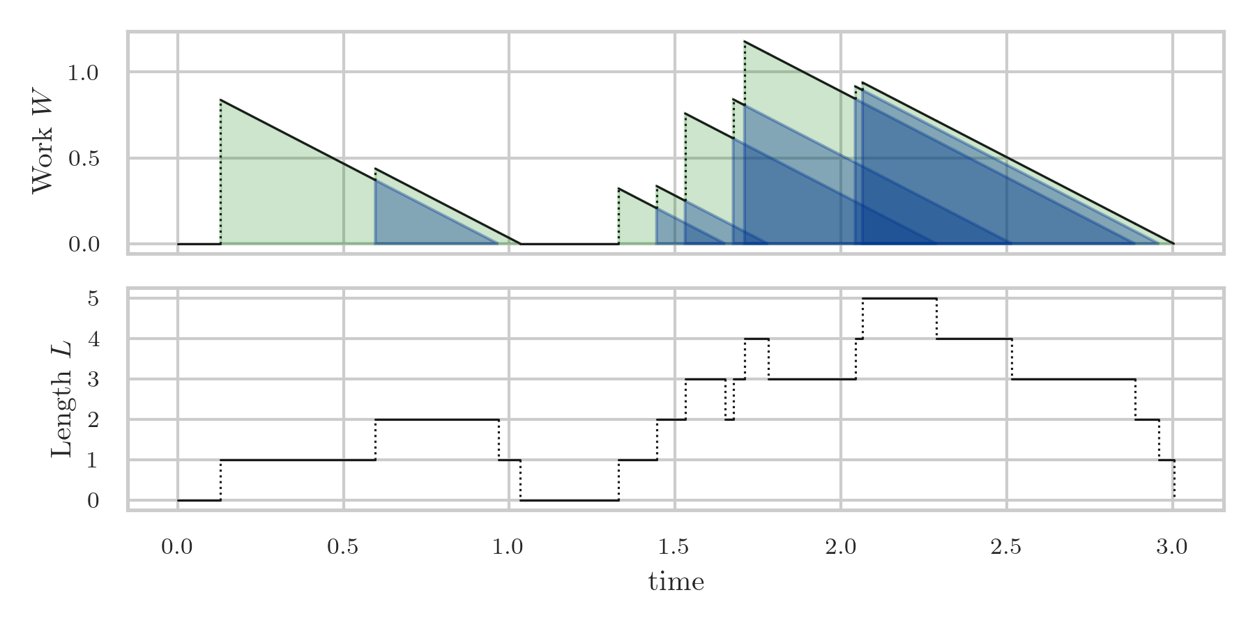
For clarity, we also want to plot vertical dotted lines to indicate that at an arrival at \(t\), the work moves from \(W(t-)\) to \(W(t)\), and downward sloping solid lines between the arrivals. Consequently, we need to be able to compute \(W(t-)\) and \(W(t)\) for arbitrary \(t\), which, in view of the definition \(W(t) = [D_{A(t)} - t]^{+}\), requires computing \(A(t-)\) and \(A(t)\). The following function uses np.searchsorted to efficiently³³ For the same reason, we used binary search in the ~RV class in Section 1.4. find the index \(k\) in an array \(a\) such that \(a_{k-1} \leq t < a_{k}\) for a given \(t\).⁴⁴ Ex 3.4.7 explains why the following function returns \(A(t)\), in particular why to subtract 1. The option right specifies the right-continuous (by default) or left-continuous version of \(A(t-)\).

def At(t, side='right'):
    "The right or left continuous version of A(t)."
    return max(np.searchsorted(A, t, side=side) - 1, 0)

From this, the work \(W(t)\) can now be implemented directly.

def W(t, side='right'):
    "The right or left continuous work in the system."
    k = At(t, side)
    return max(D[k] - t, 0)

To plot \(W\) we still need an efficient algorithm to sort chronologically arrival and departure times. For this, we use a heap queue.

A heap queue stores tuples (or lists) in a list such that the tuples (or lists) can be retrieved according to some ordering rule. Here is an example. Tuples with ages and animal names can be arbitrarily pushed onto a heap.

from heapq import heappop, heappush

heap = []

heappush(heap, (25, "Turtle"))
heappush(heap, (14, "Dog"))
heappush(heap, (18, "Cat"))
heappush(heap, (21, "Horse"))
heappush(heap, (20, "Lion"))

Popping from the heap yields the animals in lexicographical order.⁵⁵ As here the age is the first element of the tuple, the sorting is here in age.

print(heappop(heap))  # Why is it the dog?
print(heappop(heap))  # Why is it the cat?

(14, 'Dog')
(18, 'Cat')

We can also push a new animal after popping.

heappush(heap, (23, "Elephant"))  # Add Elephant

Let's pop until the heap is empty. Observe that the dog and cat are removed from the heap, due to the earlier popping.

while heap:
    e = heappop(heap)
    print(e)

(20, 'Lion')
(21, 'Horse')
(23, 'Elephant')
(25, 'Turtle')

A heap queue is algorithmically efficient: it supports pushing at our convenience while guaranteeing that elements will be popped in the correct order. Thus, it is the ideal data structure for ordering arrival and departure events that are intertwined.

With heap queues we can plot the work \(W\) and the system size \(L\) for Fig.. For \(\{L(t)\}\), we start with setting L=0 and add \(1\) when an arrival occurs, and subtract \(1\) for a departure. We therefore form a list of arrival events of type \((A_{k}, 1)\) and a second list \((D_k, -1)\) for the departures. As these lists are already sorted, merging them suffices.⁶⁶ The function merge returns a generator, not a list. However, heapify expects a list instead of a generator. We call list() to convert the generator.

arrivals = [(t, 1) for t in A[1:]]
departures = [(t, -1) for t in D[1:]]
events = list(heapq.merge(arrivals, departures))
heapq.heapify(events)

Finally, we can plot the dotted and solid lines for \(W\), and \(L\). Note that W(now, 'left') corresponds to \(W(t-)\) when the time \(t\) is now.

L, past = 0, 0
while events:
    now, delta = heapq.heappop(events)
    ax1.plot([past, now], [W(past), W(now, 'left')], c='k', lw=0.75)
    ax1.plot([now, now], [W(now, 'left'), W(now)], ":", c='k', lw=0.75)
    ax2.plot([past, now], [L, L], c='k', lw=0.75)
    ax2.plot([now, now], [L, L + delta], ":", c='k', lw=0.75)
    L += delta
    past = now

from heapq import heappop, heappush
heap = []
heappush(heap, (1.9, "Long"))
heappush(heap, (1.7, "Egg"))
heappush(heap, (1.3, "Zeno"))
print(heappop(heap))

(1.3, 'Zeno')